import numpy as np
    import pandas as pd
    import matplotlib.pyplot as plt
    import seaborn as sn
    import tensorflow as tf

 

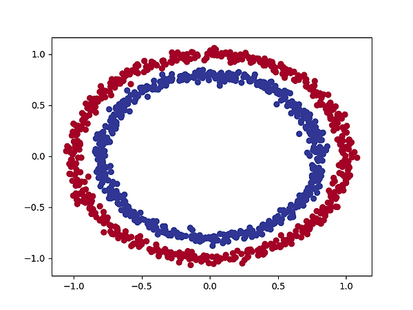
    ### Creating data.
   

    from sklearn.datasets import make_circles
    n_samples = 1200
    X, y = make_circles(n_samples, noise=0.03, random_state=42)

    circles = pd.DataFrame({"X0":X[:, 0], "X1":X[:, 1], "label":y})

   
    plt.scatter(X[:, 0], X[:, 1], c=y, cmap=plt.cm.RdYlBu)

​

​

​

​

​

​

​

​

​

​

​

​

​

​

​

​

​

​

​

​

​

​

​

​

 

    ### Split data into train, valditaion and test sets.
 

    X_train, y_train = X[:800], y[:800]
    X_val, y_val = X[800:1000], y[800:1000] 
    X_test, y_test = X[1000:1200], y[1000:1200]

 

    ### model.
   

    tf.random.set_seed(42)
    model = tf.keras.Sequential([tf.keras.layers.Dense(4, activation=tf.keras.activations.relu),
                                                    tf.keras.layers.Dense(4, activation=tf.keras.activations.relu),
                                                    tf.keras.layers.Dense(1, activation=tf.keras.activations.sigmoid)])
    model.compile(loss=tf.keras.losses.binary_crossentropy,
                              optimizer=tf.keras.optimizers.Adam(lr=0.01),
                              metrics=['accuracy'])
    history = model.fit(X_train, y_train, validation_data=(X_val,y_val), verbose=1, epochs=25)

​

    ### Evaluate the model.
    

    df = pd.DataFrame(history.history)
   

    fig1,ax1 = plt.subplots(1,2)
    ax1[0].plot(df['loss'], label='train loss')
    ax1[0].plot(df['val_loss'], label='validation loss')
    ax1[0].set_xlabel('epoch')
    ax1[0].set_ylabel('loss')
    ax1[0].set_title('Model loss curves')
    ax1[0].legend()
    ax1[0].grid()
 

    ax1[1].plot(df['accuracy'], label='train accuracy')
    ax1[1].plot(df['val_accuracy'], label='validation accuracy')
    ax1[1].set_xlabel('epoch')
    ax1[1].set_ylabel('accuracy')
    ax1[1].set_title('Model accuracy curves')
    ax1[1].legend()
    ax1[1].grid()

 

 

 

 

 

 

 

 

 

 

 

 

 

 

 

​

​

​

​

​

​

​

​

 

​
 

    loss, accuracy = model.evaluate(X_test, y_test)
    print(f"Model loss on the test set: {loss:.5f}") # Model loss on the test set: 0.05795
    print(f"Model accuracy on the test set: {100*accuracy:.2f}%") # Model accuracy on the test set: 99.50%

 

    ### Make predictions.
 

     y_preds = model.predict(X_test)
 

    ### Confusion Matrix.
   

    df = pd.DataFrame({'True':y_test,
                                     'Prediction':tf.round(tf.squeeze(y_preds).numpy())})
    confusion_matrix = pd.crosstab(df['True'], df['Prediction'], rownames=['True'], colnames=['Prediction'])
    sn.heatmap(confusion_matrix, annot=True, fmt=".1f")

 

 

 

 

 

 

 

 

 

 

 

 

 

 

 

 

 

 

​

​

 

 

 

​
 

    ### Plot the decision boundaries for the training and test sets.

 

    def plot_decision_boundary(model, X, y):
          # Define the axis boundaries of the plot and create a meshgrid.
          x_min, x_max = X[:, 0].min() - 0.1, X[:, 0].max() + 0.1
          y_min, y_max = X[:, 1].min() - 0.1, X[:, 1].max() + 0.1
          xx, yy = np.meshgrid(np.linspace(x_min, x_max, 100),
                                              np.linspace(y_min, y_max, 100))

          # Create X values (we're going to predict on all of these).
          x_in = np.c_[xx.ravel(), yy.ravel()]
         

         # Make predictions using the trained model.
         y_pred = model.predict(x_in)
         y_pred = np.round(y_pred).reshape(xx.shape)
 

        # Plot decision boundary.
        plt.contourf(xx, yy, y_pred, cmap=plt.cm.RdYlBu, alpha=0.7)
        plt.scatter(X[:, 0], X[:, 1], c=y, s=40, cmap=plt.cm.RdYlBu)
        plt.xlim(xx.min(), xx.max())
        plt.ylim(yy.min(), yy.max())

​
 

    plt.figure(figsize=(12, 6))
    plt.subplot(1, 2, 1)
    plt.title("Train")
    plot_decision_boundary(model, X=X_train, y=y_train)
    plt.subplot(1, 2, 2)
    plt.title("Test")
    plot_decision_boundary(model, X=X_test, y=y_test)

​

​

​
 

​