CNN (Tensorflow)
Summary
Building 3 different custom models for classification problem with Tensorflow.
The main goal is not build the best model, but showing different options how to build a model.
Example 1. 10 labels using Sparse Categorical Crossentropy loss function.
import numpy as np
import pandas as pd
import matplotlib.pyplot as plt
import seaborn as sn
import tensorflow as tf
from tensorflow.keras.models import Model
from tensorflow.keras.layers import Input, Conv2D, Dense, Flatten, Dropout
### Load in the data
fashion_mnist = tf.keras.datasets.fashion_mnist
(x_train, y_train), (x_test, y_test) = fashion_mnist.load_data()
x_train, x_test = x_train/255.0, x_test/255.0
### Data shape
print(x_train.shape) # (60000, 28, 28)
print(y_train.shape) # (60000,)
print(x_test.shape) # (10000, 28, 28)
print(y_test.shape) # (10000,)
labels = len(set(y_train))
print("Number of classes: ", labels) # Number of classes: 10
### Add color channel
x_train = np.expand_dims(x_train,-1)
x_test = np.expand_dims(x_test,-1)
print(x_train.shape) # (60000, 28, 28, 1)
print(x_test.shape) # (10000, 28, 28, 1)
### Labels
class_names = ['T-shirt/top', 'Trouser', 'Pullover', 'Dress', 'Coat',
'Sandal', 'Shirt', 'Sneaker', 'Bag', 'Ankle boot']
labels = dict(zip(range(labels),class_names))
print(labels)
# {0: 'T-shirt/top',
# 1: 'Trouser',
# 2: 'Pullover',
# 3: 'Dress',
# 4: 'Coat',
# 5: 'Sandal',
# 6: 'Shirt',
# 7: 'Sneaker',
# 8: 'Bag',
# 9: 'Ankle boot'}
### Plot images of fashion mnist data
plt.figure(1,figsize=(12,7))
for i in range(0,9):
ax = plt.subplot(3,3,i+1)
plt.imshow(x_train[i], cmap='gray_r')
plt.title(labels[y_train[i]])
plt.axis(False)
### Model 1
tf.random.set_seed(42)
i = Input(shape=x_train[0].shape)
x = Conv2D(filters = 32, kernel_size = (3,3), strides = 2, activation = 'relu')(i)
x = Conv2D(filters = 64, kernel_size = (3,3), strides = 2, activation = 'relu')(x)
x = Conv2D(filters = 128, kernel_size = (3,3), strides = 2, activation = 'relu')(x)
x = Flatten()(x)
x = Dense(units=512, activation='relu')(x)
x = Dense(units=len(labels), activation='softmax')(x)
model = Model(i,x)
model.compile(loss = 'sparse_categorical_crossentropy',
optimizer = 'adam',
metrics=['accuracy'])
history = model.fit(x_train, y_train, validation_data = (x_test, y_test), epochs = 15)
### Model 2
tf.random.set_seed(42)
model_1 = tf.keras.Sequential([ Conv2D(filters = 32, kernel_size = (3,3), strides = 2, activation = 'relu',
input_shape=x_train[0].shape),
Conv2D(filters = 64, kernel_size = (3,3), strides = 2, activation = 'relu'),
Conv2D(filters = 128, kernel_size = (3,3), strides = 2, activation = 'relu'),
Flatten(),
Dense(units=512, activation='relu'),
Dense(units=len(labels), activation='softmax') ])
model_1.compile(loss = tf.keras.losses.SparseCategoricalCrossentropy(),
optimizer = tf.keras.optimizers.Adam(lr=0.001),
metrics=['accuracy'])
history_1 = model_1.fit(x_train, y_train, validation_data = (x_test, y_test), epochs = 15)
### Model 3
tf.random.set_seed(42)
model_2 = tf.keras.Sequential()
model_2.add(Conv2D(filters = 32, kernel_size = (3,3), strides = 2, activation = 'relu',
input_shape=x_train[0].shape))
model_2.add(Conv2D(filters = 64, kernel_size = (3,3), strides = 2, activation = 'relu'))
model_2.add(Conv2D(filters = 128, kernel_size = (3,3), strides = 2, activation = 'relu'))
model_2.add(Flatten())
model_2.add(Dense(units=512, activation='relu'))
model_2.add(Dense(units=len(labels), activation='softmax'))
model_2.compile(loss = tf.keras.losses.SparseCategoricalCrossentropy(),
optimizer = tf.keras.optimizers.Adam(lr=0.001),
metrics=['accuracy'])
history_2 = model_2.fit(x_train, y_train, validation_data = (x_test, y_test), epochs = 15)
### Model summary
model.summary()
Model: "functional_1"
_________________________________________________________________
Layer (type) Output Shape Param #
=================================================================
input_1 (InputLayer) [(None, 28, 28, 1)] 0
_________________________________________________________________
conv2d (Conv2D) (None, 13, 13, 32) 320
_________________________________________________________________
conv2d_1 (Conv2D) (None, 6, 6, 64) 18496
_________________________________________________________________
conv2d_2 (Conv2D) (None, 2, 2, 128) 73856
_________________________________________________________________
flatten (Flatten) (None, 512) 0
_________________________________________________________________
dense (Dense) (None, 512) 262656
_________________________________________________________________
dense_1 (Dense) (None, 10) 5130
=================================================================
Total params: 360,458
Trainable params: 360,458
Non-trainable params: 0
_________________________________________________________________
### See the inputs and outputs of each layer
from tensorflow.keras.utils import plot_model
plot_model(model_2, show_shapes=True)
### Evaluate models
a = model.evaluate(x_test,y_test)
b = model_1.evaluate(x_test,y_test)
c = model_2.evaluate(x_test,y_test)
print(f' Model 1. loss = {a[0]:.5f}, accuracy = {a[1]:.5f}') # Model 1. loss = 0.49764, accuracy = 0.89530
print(f' Model 2. loss = {b[0]:.5f}, accuracy = {b[1]:.5f}') # Model 2. loss = 0.49764, accuracy = 0.89530
print(f' Model 3. loss = {c[0]:.5f}, accuracy = {b[1]:.5f}') # Model 3. loss = 0.49764, accuracy = 0.89530
### Evaluation graphs
df = pd.DataFrame(history.history)
plt.figure(2,figsize=(12,7))
df['loss'].plot(label='train loss')
df['val_loss'].plot(label='validation loss')
plt.xlabel('epoch')
plt.ylabel('loss')
plt.title('Loss VS Epoch')
plt.legend()
plt.grid()
plt.figure(3,figsize=(12,7))
df['accuracy'].plot(label='train accuracy')
df['val_accuracy'].plot(label='validation accuracy')
plt.xlabel('epoch')
plt.ylabel('accuracy')
plt.title('Accuracy VS Epoch')
plt.legend()
plt.grid()
### Confusion Matrix
y_pred = model.predict(x_test).argmax(axis=1)
df = pd.DataFrame({'True':y_test,'Prediction':y_pred})
df.replace(labels,inplace=True)
confusion_matrix = pd.crosstab(df['True'], df['Prediction'], rownames=['True'], colnames=['Prediction'])
plt.figure(4,figsize=(12,7))
ax = sn.heatmap(confusion_matrix, annot=True, fmt=".1f", linewidths=.5)
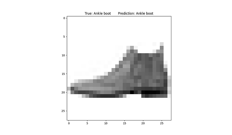
### Plot classified example
idx = np.where(y_test==y_pred)[0][0]
plt.figure(5,figsize=(12,7))
plt.imshow(x_test[idx],cmap='gray_r')
plt.title(f"True: {labels[y_test[idx]]} Prediction: {labels[y_pred[idx]]}")
### Plot misclassified example
idx = np.where(y_test!=y_pred)[0][0]
plt.figure(6,figsize=(12,7))
plt.imshow(x_test[idx],cmap='gray_r')
plt.title(f"True: {labels[y_test[idx]]} Prediction: {labels[y_pred[idx]]}")